Temporal Networks in SeriationCT

Overview

In my description of the SeriationCT model, I refer to controlling the connections and interaction intensity between communities by a diachronic “regional interaction model.” This note formalizes the way I handle specifying such models, using one type of “temporal network” formalism (Holme and Saramäki 2012).

Two types of temporal network model are in general use today. The first records the time at which events occur, where events are represented by the appearance and deletion of edges between vertices. Such “instantaneous” temporal networks are useful for modeling time series data for events whose duration is small compared to the overall dynamics. Examples include text messages between individuals or conversations at a party. The second type of temporal network model (an “interval” network) records the pattern of vertices and edges over intervals. During each interval, the adjacency matrix is assumed to be static, changing at specific time indices. This type of model is represented by an integer-indexed sequence of full adjacency matrices, and is useful for representing an evolving situation or context upon which some other dynamics plays out. In other words, interval networks are perfect for representing ongoing CT in a more slowly changing context of local community formation, contact, isolation, and abandonment.

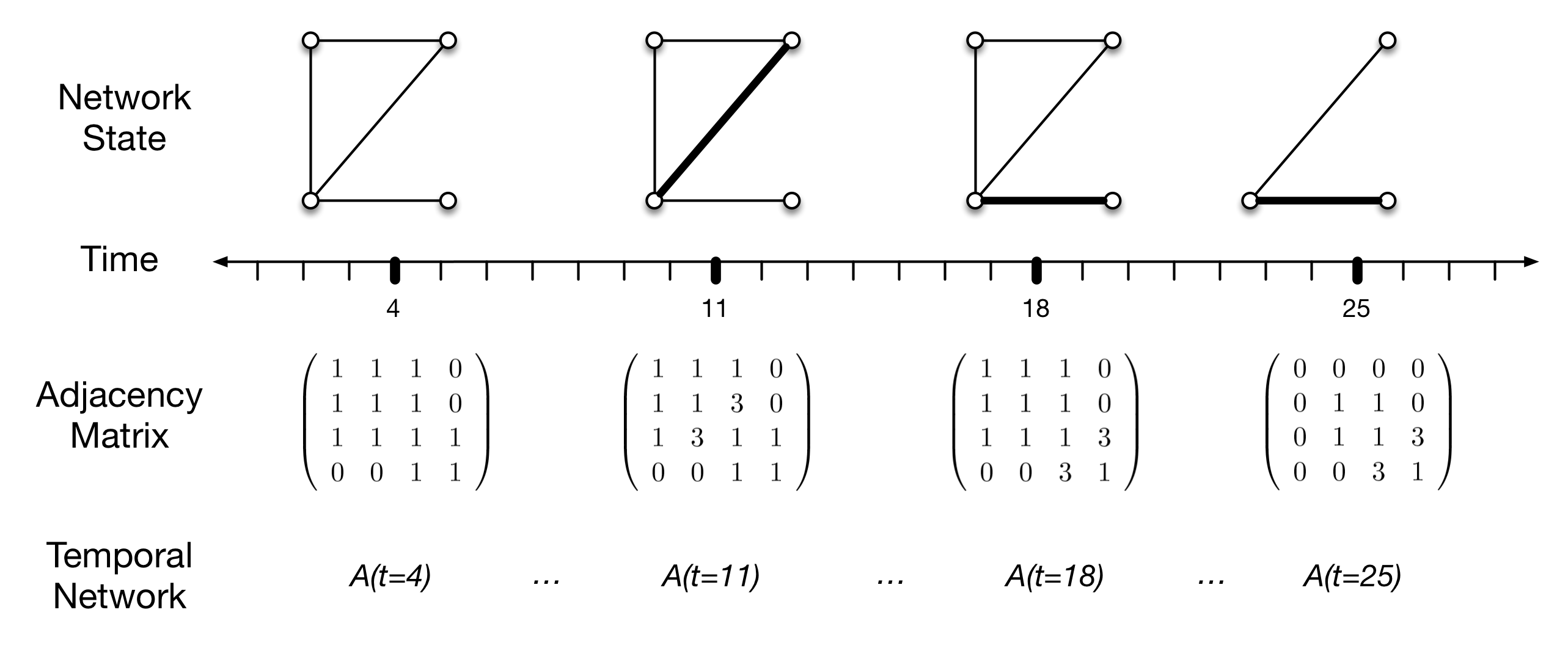
In Figure 1, I show only four vertices, to clearly demonstrate the implementation of a temporal network. Vertices here represent local communities or demes, edges (\(e_{i,j}\)) represent interaction (e.g., intermarriage, trade, or other contacts resulting in opportunities for social learning), and the thickness of the edge is a graphical depiction of edge weights (\(w_{i,j}\)) which is an ordinal measure of interaction intensity. Vertex pairs without a connecting edge are assumed not to be interacting during the time interval represented by the adjacency matrix.

The figure represents a pattern of connections (at time \(t=4\), say), and then a change at \(t=11\) to increase the intensity of interaction or learning between communities 2 and 3. This interaction declines to similar levels as other pairs of communities at \(t=18\), but interaction between communities 3 and 4 increases. Finally, at \(t=25\), community 1 is abandoned, with no other changes in the interaction pattern.

These changes are reflected in the sequence of adjacency matrices below, by the change in off-diagonal edge weights. Diagonal elements are used here to indicate the existence of a population, and thus we mark the loss of community 1 by a zero in the upper left diagonal position of the matrix (naturally, its off diagonal elements go to zero as well).

The full model is thus a sequence of tuples of the form \((t_0, A(t_0)) \ldots (t_i, A(t_i))\).

Implementation

One possibility is to go from some kind of specification (e.g., start with \(N\) vertices, generate \(M\) clusters with strong internal connectivity and weak connectivity between, at times \(T_i \ldots T_j\) vary the strength of between cluster connections, …) to a sequence of numpy arrays which represent weighted adjacency matrices.

The regional model would be characterized at any given time by a single numpy array, which represented the state of the metapopulation network at that time. At a model tick where a new network model state is supposed to arrive, the new state is substituted, and the population model remapped to match. The details for that remapping are as follows:

1. If a vertex is destroyed by a state change (detected by finding a zero on the diagonal for one of the demes/vertices), its agents are removed from the population and any edges between them and other neighbors removed.

2. If a vertex is added by a state change (detected by finding a one on the diagonal for a deme/vertex that does not currently exist in the active population), a new deme (vertex) is created, and the population size for that deme is seeded by random sampling of a neighboring deme (chosen at random from those which the new deme is connected in the regional population matrix).

3. In order to determine connectivity changes (as opposed to new or lost vertices), we have to compare the new and old numpy arrays. This is easily done using numpy.equal(), which produces an array of the same dimension filled with booleans that indicate positions which are equal. In this case, we would find any instances of False in the upper diagonal portion of the array, and modify their weight.

Modification of the “weight” between two vertices means changing the number of individuals who have edges between the two vertices. This could be chosen at random.

import numpy as np
t1 = np.array([[1,1,1,0],[1,1,1,0],[1,1,1,1],[0,0,1,1]])
t2 = np.array([[1,1,1,0],[1,1,3,0],[1,3,1,1],[0,0,1,1]])
np.equal(t1,t2)

ud = np.triu_indices(4)

difference_t1_t2 = np.equal(t1,t2)
difference_t1_t2[ud]

Changes to the upper-triangular portion of the matrix, above the diagonal are thus indicative of changes in weight between two nodes. We can find the indices of the demes for which this occurs easily:

# t1 and t2 arrays as before
# returns tuple where element 0 is a list of row coordinates
# and element 1 is a list of column coordinates
changed_edges = np.nonzero( np.triu( t2 - t1 ))

Changes to the existence of demes are modeled on the diagonal of the adjacency matrix. In the following, deme 0 goes away, thus yielding a zero in the \(0,0\) position of the adjacency matrix, and corresponding off-diagonal entries go to zero because edges are lost when a deme is removed (of course). In contrast, between time steps 1 and 2, no demes enter or exit.

t3 = np.array([[0,0,0,0],[0,1,1,0],[0,1,1,3],[0,0,3,1]])

np.nonzero(np.diagonal( t2 - t1 ))
# result is (array([], dtype=int64),)

np.nonzero(np.diagonal( t3 - t2 ))
# result is (array([0]),)

# subtracting the two arrays and accessing the diagonal element for index 0 
# gives us the DIRECTION
t3_t2 = t3 - t2
t3_t2[0,0]  
# answer is -1

A negative element on the diagonal of the differenced array indicates that the deme at that index is exiting the model at that time step. A positive element on the diagonal thus indicates a new deme entering the model at that time step.

References Cited

Holme, Petter, and Jari Saramäki. 2012. “Temporal Networks.” Physics Reports 519 (3). Elsevier: 97–125.