Loss Functions for ABC Model Selection with Seriation Graphs as Data

Background

Traditional archaeological seriation generated solutions that always had a static linear order, either by use of a multidimensional scaling algorithm or via Fordian manual shuffling of assemblages. In such context, departures from a “correct” solution can be measured by the number of “out of order” assemblages (or via a more opaque “stress” statistic in some cases).

Last year Carl Lipo and I introduced a method for finding sets of classical Fordian seriations from a set of assemblages via an agglomerative iterative procedure (Lipo 2015). We called the resulting seriations “iterative deterministic seriation solutions” or IDSS. IDSS is capable of using any metric for joining assemblages, including classic unimodality, or various distance measures (something we’ll be talking about at the SAA meetings this year).

When IDSS finds groups of data points that seriate together, but do not seriate (within thresholds) with other groups of points, several solutions are created rather than forcing all of the data points into a single scaling or solution (as has been typical practice with statistical seriation by archaeologists in the past). Instead, IDSS outputs all valid solution sets, since the discontinuities between solution sets may indicate lack of cultural interaction, poor recovery sampling of the archaeological record, or other real-world factors.

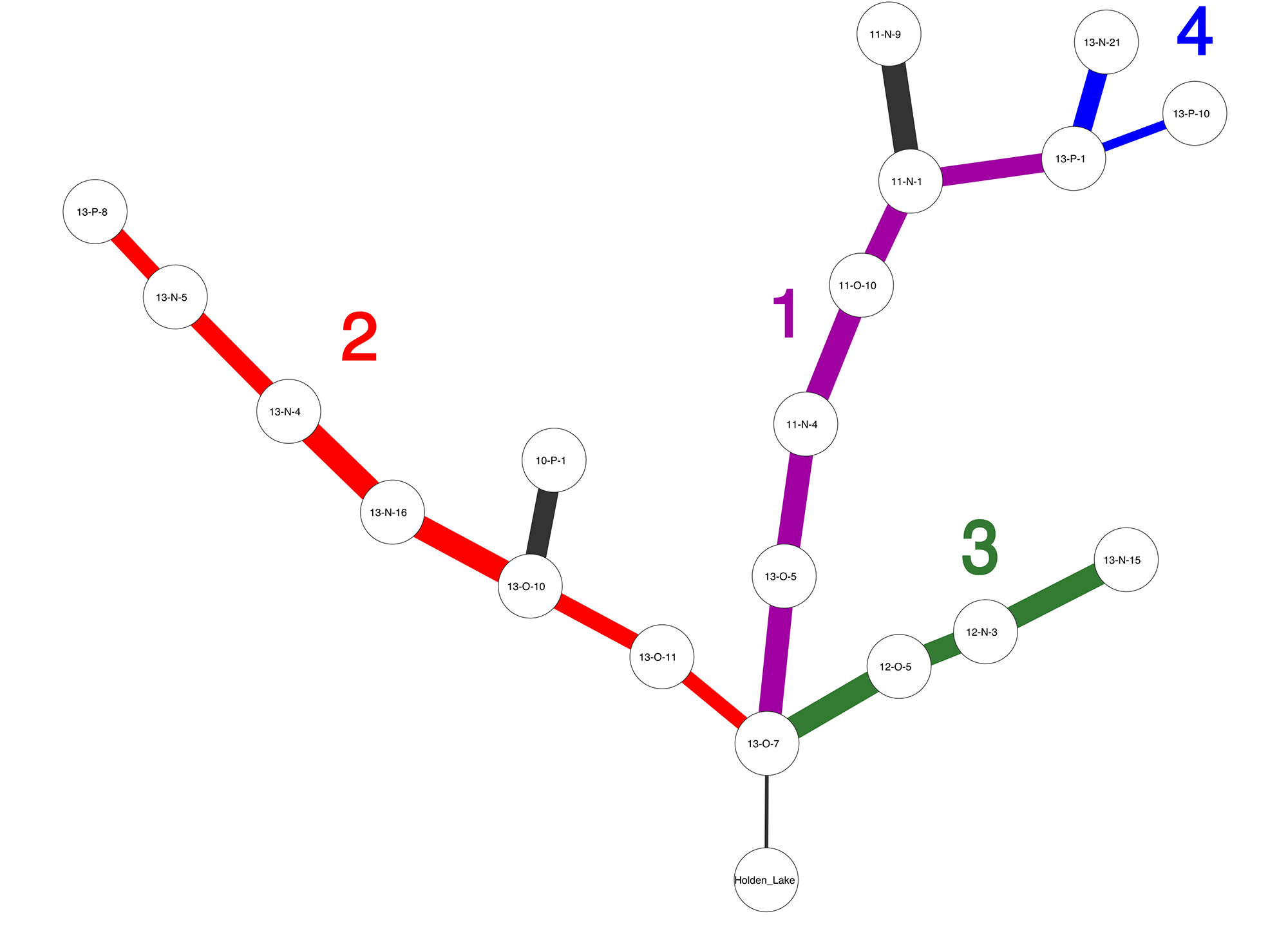
Frequently, one assemblage or data point will occur in multiple solutions, and when this occurs IDSS overlays the solutions and forms a tree. From our paper, Figure 1 shows an IDSS frequency seriation solution for archaeological sites in the Central Mississippi River Valley. Each assemblage is represented by decorated ceramic class frequencies, and we can see that there are at least three major solutions which share assemblage 13-O-7, and a number of minor branches.

The Problem

My current research is aimed at developing ways of treating IDSS seriation solution graphs as data points in machine learning algorithms, with the goal of fitting coarse grained, regional models of cultural transmission and information diffusion to our data. Seriations are the perfect tool for capturing regional-scale social influences that are time-transgressive.

There are several challenges in this work. The first, which is described in a previous post is to create regional metapopulation models with cultural transmission that yield seriations, rather than just type or variant frequencies, as their observable output.

The second challenge is then to find an inferential framework for model selection which allows one to measure the goodness-of-fit between the theoretical model’s output, and specific empirical seriations like Figure 1.

This second challenge is perfectly suited to an Approximate Bayesian Computation approach (Beaumont, Zhang, and Balding 2002; Csilléry et al. 2010; Marin et al. 2012; Toni et al. 2009), since while we can simulate data from each social learning model, writing down the likelihood function for each model is generally an intractable problem.

In brief, ABC model selection involves simulating a large number of synthetic data points from each model, calculating summary statistics from those data points, measuring the distance (losses) between summary statistics and observed data, and choosing the model whose losses are the smallest.

In my current work, the “models” are actually a combination of:

1. A social learning model (e.g., unbiased cultural transmission or conformist transmission)
2. Parameters for that social learning model (e.g., innovation rates)
3. A spatiotemporal population model that describes how communities evolved in a region and what the pattern of community interaction was over time

This is a fairly complex “model” to fit, but we can easily simulate samples of cultural variant frequencies across subpopulations from each model (using the SeriationCT software suite, and then use IDSS to seriate those variant frequencies, yielding simulated versions of Figure 1.

What we need, then, is a way to measure the distance or loss between Figure 1 and various simulated seriation graphs. Once we have a good loss function, we should be able to perform ABC model selection on seriation graphs.

Distance/Loss for Unlabelled, Unordered Graphs

In general, we want a function which measures the structural similarity of two graphs. There are many approaches to the problem (see (Zager and Verghese 2008) for a review). Graph edit distance would be a fairly natural metric, but most algorithms for edit distance rely on matching node identities, and many algorithms also rely upon graphs being ordered as well as labelled.

The simulated seriations which come out of the SeriationCT package are unlabelled, and we can’t label them with the identities of the assemblages in our empirical data. So our loss function has to measure structural similarity without reference to node identity, or any notion of ordering or orientation for the graphs.

This leads fairly directly to using purely algebraic properties of the seriation graphs, and in particular the spectral properties of various matrices associated with the graphs. We know that the eigenvalues of the (possibly binarized) adjacency matrix are related to the edge structure of a graph, and that the eigenvalues of the Laplacian of the adjacency matrix are an even more sensitive indicator of structure (Godsil and Royle 2001).

In a technical report, Koutra et al. (Koutra et al. 2011) suggest using the sum of squared differences between the Laplacian spectra of two graphs, trimming the spectra to use only 90% of the total eigenvalue weight. This is attractive from a statistical perspective, essentially giving us the L2 loss between Laplacian spectra for two graphs.

Given adjacency matrices \(A_1\) and \(A_2\) for graphs \(G_1\) and \(G_2\), the Laplacian matrix is simply \(L_1 = D_1 - A_1\) and \(L_2 = D_2 - A_2\), where \(D_i\) are the corresponding diagonal matrix of vertex degrees. The spectrum is then the set of eigenvalues \((\lambda_1 \ldots \lambda_n)\). Since the Laplacian is positive semi-definite, all of the eigenvalues in the spectrum are positive real numbers. It is possible to put some bounds on the eigenvalues, and thus predetermine the range of possible loss function values for graphs with a given number of vertices, but I leave that to a future post.

If we use the full spectrum of values, our L2 spectral loss function is then:

\(\mathcal{L}_{sp} = \sum_{i=1}^{n} (\lambda_{1i} - \lambda_{2i})^2\)

and if we only use a trimmed set of eigenvalues (say, those which contribute to the top 90% of the total sum of the spectrum), we sort the list of those \(k\) eigenvalues and replace \(n\) with \(k\) in the previous equation.

Implementation

In Python, we can implement this loss function for NetworkX graph objects as follows (now part of the seriationct.analytics module):

import networkx as nx
import numpy as np

def graph_spectral_similarity(g1, g2, threshold = 0.9):
    """
    Returns the eigenvector similarity, between [0, 1], for two NetworkX graph objects, as
    the sum of squared differences between the sets of Laplacian matrix eigenvalues that account
    for a given fraction of the total sum of the eigenvalues (default = 90%).

    Similarity scores of 0.0 indicate identical graphs (given the adjacency matrix, not necessarily
    node identity or annotations), and large scores indicate strong dissimilarity.  The statistic is
    unbounded above.
    """
    l1 = nx.spectrum.laplacian_spectrum(g1, weight=None)
    l2 = nx.spectrum.laplacian_spectrum(g2, weight=None)
    k1 = _get_num_eigenvalues_sum_to_threshold(l1, threshold=threshold)
    k2 = _get_num_eigenvalues_sum_to_threshold(l2, threshold=threshold)
    k = min(k1,k2)
    sim = sum((l1[:k] - l2[:k]) ** 2)
    return sim


def _get_num_eigenvalues_sum_to_threshold(spectrum, threshold = 0.9):
    """
    Given a spectrum of eigenvalues, find the smallest number of eigenvalues (k)
    such that the sum of the k largest eigenvalues of the spectrum
    constitutes at least a fraction (threshold, default = 0.9) of the sum of all the eigenvalues.
    """
    if threshold is None:
        return len(spectrum)

    total = sum(spectrum)
    if total == 0.0:
        return len(spectrum)

    spectrum = sorted(spectrum, reverse=True)
    running_total = 0.0

    for i in range(len(spectrum)):
        running_total += spectrum[i]
        if running_total / total >= threshold:
            return i + 1
    # guard
    return len(spectrum)

References Cited

Beaumont, Mark A, W Zhang, and D J Balding. 2002. “Approximate Bayesian computation in population genetics.” Genetics. http://www.genetics.org/content/162/4/2025.short.
Csilléry, Katalin, Michael G B Blum, Oscar E Gaggiotti, and Olivier François. 2010. “Approximate Bayesian Computation (ABC) in practice.” Trends in Ecology & Evolution 25 (7): 410–18. https://doi.org/10.1016/j.tree.2010.04.001.
Godsil, Christopher David, and Gordon Royle. 2001. Algebraic Graph Theory. Vol. 8. Springer New York.
Koutra, Danai, Ankur Parikh, Aaditya Ramdas, and Jing Xiang. 2011. “Algorithms for Graph Similarity and Subgraph Matching.” Technical Report of Carnegie-Mellon-University.
Lipo, Mark E. AND Dunnell, Carl P. AND Madsen. 2015. “A Theoretically-Sufficient and Computationally-Practical Technique for Deterministic Frequency Seriation.” PLoS ONE 10 (4). Public Library of Science: e0124942. https://doi.org/10.1371/journal.pone.0124942.
Marin, Jean-Michel, Pierre Pudlo, Christian P Robert, and Robin J Ryder. 2012. “Approximate Bayesian Computational Methods.” Statistics and Computing 22 (6). Springer: 1167–80.
Toni, Tina, David Welch, Natalja Strelkowa, Andreas Ipsen, and Michael P H Stumpf. 2009. “Approximate Bayesian computation scheme for parameter inference and model selection in dynamical systems.” Journal of Royal Society Interface 6 (31). The Royal Society: 187–202. https://doi.org/10.1098/rsif.2008.0172.
Zager, Laura A, and George C Verghese. 2008. “Graph Similarity Scoring and Matching.” Applied Mathematics Letters 21 (1). Elsevier: 86–94.