Time Averaging and the CT Mixture Model

Created: 09 Jul 2014

Modified: 23 Jul 2020

BibTeX Entry

RIS Citation

Print

Adding Time Averaging to the CT Mixtures Model

At present (v1.0, May 2014), the ctmixtures model performs the following sampling of the evolving population:

1. Counts and frequencies of traits for \(M\) features/loci across the population.
2. Counts and frequencies of traits for \(M\) features/loci at a list of sample sizes (e.g., 20, 50, 100)
3. Trait survival analysis for an interval \(T\), calculated for the last \(T * N\) ticks of the simulation, given population size of \(N\).

What version 1.0 did not include is:

1. Time averaged observations of trait counts and frequencies over a list of durations
2. Calculation of trait survival for an interval \(T\), where the starting and finishing samples are both time averaged.

Simulation Event Timing

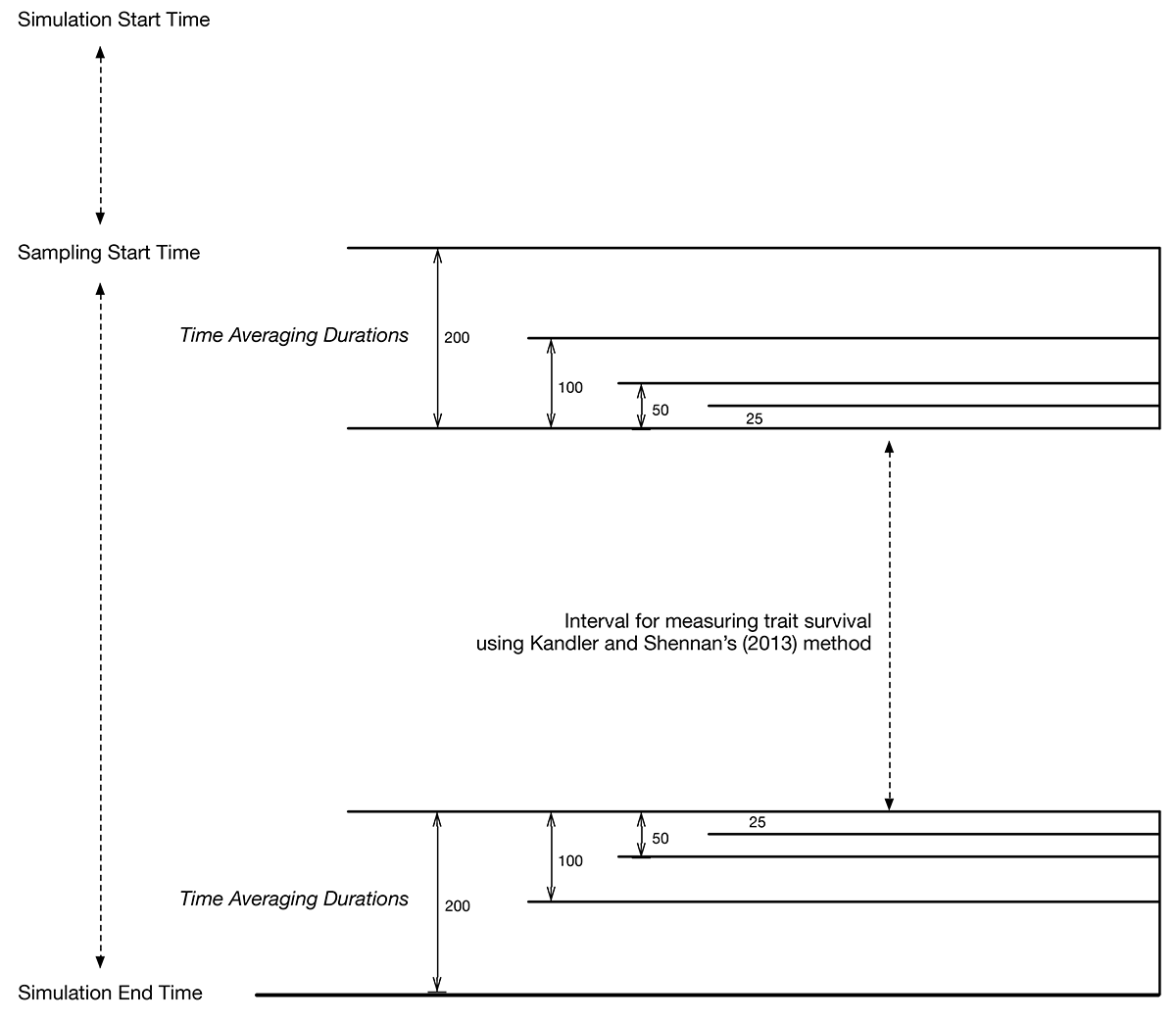
The following diagram shows how time averaging is integrated into the simulation event stream. Time runs from top (start of simulation) to bottom (end of simulation). Between simulation start time and the start of sampling, the population is evolving from its initial condition to quasi-stationarity. Sampling start time is calculated to occur at a multiple of the expected mixing time, to ensure that the population is at quasi-equilibrium.

In the center of the diagram is an interval, marked with a dotted vertical line, depicting the interval over which we track the survival of traits given (Kandler and Shennan 2013).

Above this fixed interval, we take one sample (of duration 1 tick) to begin the survival analysis, and below the interval, a sample of duration 1 to complete it. This sample is directly comparable to the analysis performed in Kandler and Shennan’s paper (although run with Moran versus Wright-Fisher dynamics).

Expanding away from this interval on both sides are a series of samples taken with greater duration. The first is a sample of duration 25, to start and finish the survival analysis, then 50 ticks, 100, and finally 200 ticks. Each pair of samples measures the trait survival when the samples are necessarily of non-trivial duration (and thus time averaged).

In addition, for the “ending” time averaged sample, I also record raw trait counts, frequencies, and other assemblage statistics, as I do with non-time averaged samples.

References Cited

Kandler, Anne, and Stephen Shennan. 2013. “A Non-Equilibrium Neutral Model for Analysing Cultural Change.” Journal of Theoretical Biology 330. Elsevier: 18–25.