Experiment - Statistical Power of Slatkin Exact vs Conformism

Created: 01 Oct 2012

Modified: 23 Jul 2020

BibTeX Entry

RIS Citation

Print

Montgomery Slatkin proposed an “exact test” (in the sense of enumeration of exact probability for an observation) for neutrality of a sample of N individuals, in which K alleles are observed (Slatkin 1994, 1996). The test calculates the probability of getting a sample of alleles “more extreme” than the observed data from the Ewens Sampling Formula (or Distribution). By way of review, the ESD gives the distribution of alleles in a sample of fixed known size, from a population at quasi-stationary equilibrium, characterized by the Wright-Fisher infinite-alleles model or its close relations. The Slatkin (or Ewens) exact test is two-tailed, and a sample can fall outside the chosen critical region (at a given alpha level) either by having too few rare alleles, or far too even a distribution.

Since the Slatkin/Ewens test does not rely upon specific details of a genetic system, it is potentially ideal for testing neutrality in CT modeling. However, its statistical power against alternative models can be limited. Lansing et al. 2008 measured power against an alternative hypothesis of male dominance and non-random mating, for example.

In the present experiment, the goal is to understand the power of the Slatkin/Ewens test against alternative models of conformist (and anti-conformist) transmission, given that a number of archaeological studies have attempted to distinguish between neutral and conformist transmission using artifact class frequency data.

Experimental Setup

• As far as I can tell, all archaeological applications of “conformist” models use the following algorithm: ** With probability c, an individual will adopt the most (or least) common trait in the population ** Otherwise with probability 1 - c, the individual will employ unbiased copying ** With probability mu, the individual acquires a brand-new trait not seen in the population previously. ** This is only one way of modeling conformist transmission, and may affect the results.
• This “Global Most Common” conformist model was implemented in TransmissionFramework.
• Simulate populations of 2000 well-mixed individuals, at theta values of 0.5, 0.75, 1.0, 3.0, 5.0, 7.0, and 9.0.
• Four levels of the “conformism factor” were simulated: 0.01, 0.005, 0.001, and 0.0005. This corresponds to 20, 10, 2, and 1 individual per generation (on average) exhibiting conformist copying. This is the “strength” of the conformist bias to transmission.
• For each combination of parameters, 3 duplicate simulation runs were made, with different random seeds.
• For each simulation run, the simulator ran for 30,000 steps. Data collection began after 10,000 steps to ensure that even with low innovation rates, the simulation was at quasi-stationary equilibrium. This is serious overkill for theta >= 1.0, but necessary for very low innovation rates since the mixing time can be long (and requires a full analysis given (Watkins 2010), not just the simplified heuristic).
• This yielded 20K independent data points for each of 3 runs per parameter combination, or 60K data points per parameter combination.
• Time averaging windows were also calculated for trait counts, with the maximum window being 3000 generations, thus yielding 10 windows per simulation run, 20 windows for aggregation at 1500 generations, down to windows at 3 generations.
• For each raw data point (all 60K per parameter combination), and for each time-averaging window, a sample of size 50 individuals was taken from the population, and their traits tabulated and recorded for input to the Slatkin Exact program.
• Samples were fed to the Slatkin exact program (see below) and the P_E value recorded. The resulting data set comprised 3.153 million Slatkin Exact test observations across all parameter values.
• All simulation data was then input to R for analysis.

Analysis

Statistical power is the converse of the probability of Type II error. In other words, it is the probability of not committing a Type II error, or a “false negative”). It measures the ability of a statistical test, in other words, to correctly detect data which derive from a process other than the data generating process designated as the “null hypothesis.”

In general, the “golden rule” is generally that a 5% probability of Type I error should be matched with a 20% probability of making a Type II error, which translates into a test with 80% power. This gives a 4:1 tradeoff between Beta-risk and Alpha-risk. This is pure convention. But since the Slatkin test reports the exact tail probability of its result, and we can similarly calculate the exact fraction of conformist samples that PASS the Slatkin test at a given alpha level, we don’t have to rely on convention and can examine directly how power changes as we vary:

• Conformism probability or rate
• Innovation rate in the population
• Duration of time-averaging (including no time averaging at all)

R code for the analysis will be available on github when the analysis is complete (9/27/12).

Results

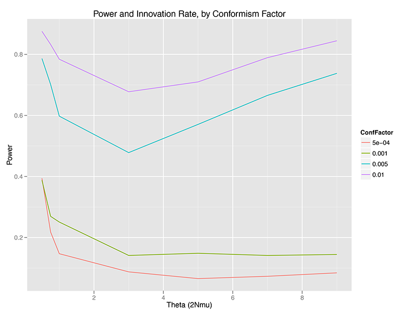
Without Time Averaging

Without any temporal aggregation, we can see that the Slatkin test can be relatively powerful for detecting conformist violations of the neutral assumptions underlying the Ewens Sampling Distribution, but only under certain conditions:

• Power is highest at very low (theta < 1.0) or relatively high (theta > 5, approximately), at least at sample size 50 (sample fraction 2.5% of the population). There is a minimum for power between 1.0 < theta < 4.0, approximately speaking. (WHY?)
• Power increases monotonically with conformism probability, at any given theta value. This makes sense – the more strongly a population is choosing the most common trait, the less the distribution of traits in a sample will look like a random draw from the ESD.
• There may be a critical point where power collapses, or I may have just chosen a progression of conformism probabilities that look separated on the graph (OPEN QUESTION).

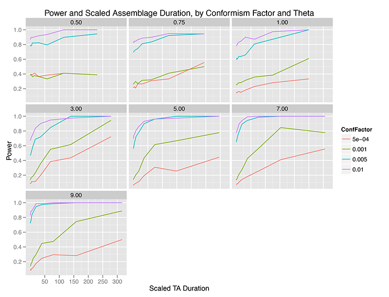
With Time Averaging

When we aggregate observations over time, the picture is intriguingly different. The x-axis below is scaled duration of observation aggregation, where the duration of aggregation is divided by the mean lifetime of traits at that level of theta (innovation rate). This helps us visualize the time scale of aggregation in something other than arbitrary simulation units.

Immediately, we can see that temporal aggregation of observations from the “Global Most Common” model of conformism increases the power of the test. Apparently, as we pile up observations, our fixed sample of individuals come more and more to reflect a very different distribution of traits than the Ewens Sampling Distribution.

This effect is, of course, sharp and pronounced at higher levels of the conformism probability, such that at almost any level of innovation, if we have reason to believe that conformism is strong in a population, the Slatkin test is nearly 100% powerful in detecting it (even though, in my earlier 2012 paper, time averaging increases the chances of a Type I error which would lead one away from a conclusion of conformism).

At weaker levels of conformism, it takes relatively large amounts of time averaging to increase the power of the test, and only at innovation rates above 3.0 do we reach the usual 80% power which is taken to mark a test capable of distinguishing between hypotheses.

Slatkin Exact Test code

Montgomery Slatkin’s original C code: CODE

The original C code for Slatkin’s monte carlo version required that the input data be coded into the source, and then compiled anew for each data value. In order to automate doing many, many exact tests for this and related studies, I modified Slatkin’s original program to take all input on the command line, and producing abbreviated output (there are several versions) to make scripting and integration into R easy. Code is at:

Madsen’s modified source code

References Cited

Slatkin, M. 1994. “An Exact Test for Neutrality Based on the Ewens Sampling Distribution.” Genetical Research 64 (01). Cambridge Univ Press: 71–74.
———. 1996. “A Correction to the Exact Test Based on the Ewens Sampling Distribution.” Genetical Research 68 (03). Cambridge Univ Press: 259–60.
Watkins, J.C. 2010. “Convergence Time to the Ewens Sampling Formula.” Journal of Mathematical Biology 60: 189–206.